

Pricing the derivatives in an AI compute stack is easier than it looks.
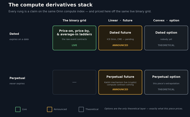
Two weeks ago I argued that compute finally gave prediction markets something they’d never had. Not a zero-or-one probability, but a real price. Dollars per GPU-hour. That’s the underlying the options playbook always wanted. Last week I laid the instruments out as one stack sitting on the binary ladder with dated and perpetual futures and options. Both times I was talking about what could be built.
This week I want to build it, at least with real numbers. Fortunately, you only have to model a few. The ladder of yes/no markets the exchange already quotes is a full probability distribution. Once you have that, most of the stack prices itself. No Black-Scholes, no volatility input. Let me walk it one number at a time, off a single late-July pull of the Kalshi H200 markets.
The ladder is already a distribution
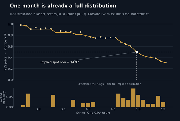
Start with one settlement date. Kalshi lists a ladder of threshold markets on it. Will an H200-hour clear $4.50? $5.00? $5.50? One yes/no contract at each strike. Every dot on the curve is one of those real, tradeable markets, and its price is just the market’s probability. The $5.00 contract trading around 48¢ means the market gives a 48% chance the price finishes above $5.00.
That single column of prices is already everything. Read straight down, it’s the odds of clearing each level. Now subtract the prices of two neighboring strikes to get the range probability. If “$4.50” trades around 70¢ and “$5.00” around 48¢, the chance the price lands between $4.50 and $5.00 is just 70 minus 48, or 22%. Do that for every pair and the column of contract prices becomes a full bar chart of where the market thinks the price will settle. The strike where the odds cross 50% is the implied spot; right now it’s about $4.98.
Why no implied volatility?
The probability distribution is the crux of the whole operation. If you’re familiar with pricing equity options, the bulk of complexity comes from modeling the implied distribution of terminal values of the underlying based on expected/implied volatility and other factors. This skips all of that and allows you to calculate the expected value with simple arithmetic since the market is already giving you distribution ranges.
For the $5.00 call, walk each bar above $5.00 and multiply how likely it is by what the call would pay there. A band around $5.25 pays $0.25, one around $5.75 pays $0.75, and so on. Multiply each payoff by that band’s probability and add them up. A put is the same sum over the bars below the strike. No model. No volatility guess. You’re weighting real payoffs by the market’s own probabilities.
Okay, maybe it’s not quite that simple. First, the bars are coarse. Strikes are listed only every fifty cents or so, so inside a band you’re assuming the price sits in the middle. Also, the ladder ends. It’s possible for the terminal value of the underlying to land way above the highest strike.
Fortunately, the structure of the Kalshi binaries helps us out here. The long-term prediction markets are monthly averages, which is good enough for long-term projection. For the near-term, where granularity means a lot more, we get weekly and monthly ladders that combine for strike widths as narrow as ten cents.
Testing it out with real data
Let’s price some options using data pulled on July 27. I’ll use the next clean weekly settling August 7. I’m skipping the current week’s (July 31) expiration since only a few days are left and its spreads are wide and its upper tail is fat. August 7 has tight quotes and a thin tail, so its average is a tighter, more reliable number. Add that ladder up and the August 7 future comes to about $4.71.
The options use the same ladder. The $5.00 call is the odds-weighted payoff above $5.00, which is about $0.16. The $5.00 put is the same sum over the bars below, about $0.45. The two aren’t independent. The call comes in 29 cents under the put, and that gap is exactly the strike, $5.00, minus the future, $4.71. That’s put-call parity. It’s out of my hands. We get it for free because both prices come from the same distribution.
Dealing with the practical long-term challenges
If we line up every month’s ladder, their centers trace a price curve across time. However, out in the far months the averaging method used above stops behaving because a critical mass of the probability sits above the highest listed strike. You can’t compute it from public prices anymore, so for the curve we’ll switch to the median, which is the 50/50 line. It only needs to know where the middle sits, and the middle is always well inside the quoted strikes.
The shape tells its own story. It isn’t the steep climb you’d expect from a chip that ran up something like 90% in the spring (like the B200). It’s roughly flat, low-to-mid $4s all the way out. What’s dramatic is the band around the line in the chart below. That’s the middle 50% of outcomes, with a 25% chance below its lower edge and 25% above its upper. Even after you throw away the extreme quarter on each end, the middle half still spans two to three dollars a year out. The line is almost irrelevant because the width is the real story. The market is pricing an enormous amount of uncertainty it has no way to offload today. Quick caveat: these far-month books are thin, so read the exact width as directional, not precise.
The one place we need a model
Two perpetual instruments sit on top of all this: the future and its options. The perpetual future is the easy one. It’s continuous exposure to the compute price that never expires and never rolls. Instead of settling, longs and shorts trade a small ongoing funding payment that keeps it tethered to spot. There’s nothing new to price. It tracks the near-dated number, about $4.98, with funding set by what the curve implies about drift.
The perpetual option refresher
Even most experienced options investors haven’t worked with perpetual options, so let’s take a moment to refresh. The most important difference between perpetual options and vanilla options is the nature of the cash flow. They’re more like perpetual futures in that you never actually buy or sell anything. Instead, the options have a market price (mark price) and you put up margin to cover a calculated risk for your long or short position.
Once your position is open, you start paying or receiving a funding payment calculated from the difference between the option’s mark and its underlying theoretical value (index price or payoff). This funding mechanism continuously anchors the trading price to its fair value.
When trading demand drives the option’s price above its theoretical value, the funding rate becomes positive, forcing long position holders to pay short position holders. Conversely, when the option trades at a discount, shorts pay longs. This ongoing exchange of cash flows replaces the traditional expiration date, allowing traders to maintain their options exposure indefinitely without the need to roll over contracts.
Anchoring to a tenor
The perpetual option is the only instrument that won’t price itself as cleanly as the others covered. But you already know the shape of it if you have experience with basic option income strategies. It’s like rolling short puts or the wheel, but on autopilot.
When you deploy a rolling option strategy like the wheel, you select a target time horizon—or anchor tenor—and continually roll expiring contracts to maintain that exposure. A perpetual option automates this concept by synthetically holding a blend of multiple expirations simultaneously. In a perpetual contract, the primary variable is the anchor tenor itself. This defines where the contract effectively sits on the volatility curve, matching the risk profile of a traditional one-month or three-month horizon, for example.
When the anchor is short, the contract behaves like rolling monthlies, where near-term vol drives the position. The mark is cheap and the funding runs fast, similar to the way theta burns when you keep rebuying the front.
When it’s longer, it’s like rolling something dated. Volatility gets more room to play out, so the day-to-day is calmer, and the mark is richer while the funding bleeds slowly.
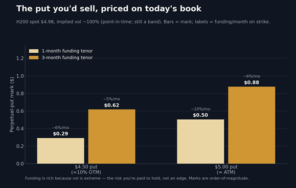
Both are the same position with a different cash-flow profile. Tenor is fixed by whoever lists the contract, so it’s the same for everything across the board. Since these compute perp options don’t exist yet, the chart below illustrates both one-month and three-month versions as examples.
Pricing perpetual options
The funding is the roll. Once you open your position you don’t need to actively manage it. You hold it and pay or receive a steady fee that stands in for the premiums you’d have spent rolling. At the one-month tenor, a $4.50 perpetual put marks around $0.29 and throws off roughly 6% a month on the strike. The exact build is a funding-weighted strip across every tenor, Paradigm’s “everlasting options”.
The whole stack, priced
Let’s step back for a second and walk through a sampling the various instruments covered here.
- YES for “Will the H200 cost more than $5.00 on August 7?” costs 0.40.
- NO for “Will the H200 cost more than $5.00 on August 7?” costs 0.60.
- The August 7 future is 4.71.
- The August 7 $5.00 call costs 0.16.
- The August 7 $5.00 put costs 0.45.
- The perpetual future costs 4.98.
- The perpetual $5.00 call costs 0.48.
- The perpetual $5.00 put costs 0.50.
That’s a lot of ways to trade compute for next week.
Summing it up
Besides the obvious reminder that much of what’s been discussed here isn’t even on anyone’s roadmap, I also want to point out that having something be priceable does not ensure it’ll be profitable. This was a fun exercise to get an idea of what these kinds of instruments would cost, but it doesn’t mean the equity options playbook will cleanly translate.
Another important unknown is whether and where the demand will be. Fortunately, demand anywhere in the stack can help drive liquidity everywhere else due to the deeply interdependent nature of the instruments. You could find yourself hedging a multi-leg perp strategy with a combination of long 9-month calls and NO 3-month binary contracts. The flexibility to express these kinds of incredibly precise views doesn’t exist anywhere else.
And, to be realistic, it doesn’t even exist here yet, either. Kalshi is working its way through binaries and perp futures while CME and ICE are working on dated futures and options. Neither has mentioned perp options so far.
And the tooling? Well, that’s a tale for another day…
