Historically, earnings announcements have played a prominent role in moving stocks. As a result, they represent the greatest known unknown in the world of investing. While projections and expectations are effective tools in modeling the direction and magnitude of equity plays, the world of options opens a new realm of opportunities based on trading volatility. After all, implied volatility (IV) scales with the unknown, so knowing when to capitalize on mispriced options can yield some great returns.

A PDF version of this article is available here.

Goals

Our goals here are to use data to help answer some of the frequently asked questions about trading earnings with options, including:

• Why trade options around earnings?
• How are earnings options priced?
• What about trading earnings directionally with options?
• How do we compare returns of long and short strategies?
• How important is option liquidity?
• What is implied volatility crush (IV crush)?
• What is earnings IV crush?
• How much does IV crush after earnings?
• Can we predict the earnings IV crush?
• Can we infer anything from the volatility surface?
• Can we still lose by selling overpriced IV?
• How can we hedge against directional moves?
• How do calendar trades hedge out directional risk?
• How can we employ calendar trades to capitalize on IV crush?
• How does this analysis hold up across the broader market?

Why trade options around earnings?

Implied volatility correlates with the demand for buying and selling options. Given the uncertainty around earnings announcements, traders often turn to buying calls and puts in order to speculate and/or insure their positions going into earnings. The market generally has a bias for buying—as opposed to selling—options for two reasons:

1. Speculators are looking to place leveraged trades with capped downsides, so buying calls or puts provides them with the defined risk/reward potential that efficiently express their views.
2. Those looking for insurance are usually hedging against equity or option positions that need to scale with the size of a potential move. As a result, they need as much option upside as they can get in order to cover the scenarios they’re hedging against.

How are earnings options priced?

This buy-side demand results in market makers ending up with books that are net short both calls and puts. This drives up the price of options, resulting in increasing IV until it finds an equilibrium relative to the overall market’s expected move. As the earnings date approaches, the at-the-money (ATM) IV for the nearest-term options is the most accurate proxy for the market’s expected post-earnings move.

Another way to look at the expected move is to price an ATM straddle made up by pairing the ATM call and put. The expectation is that this straddle should break even, so the combined premium is the implied move the market expects after the earnings announcement. If IV were too low, then there would be more buying pressure to drive the IV up. If it were too high, selling pressure would drive it down.

A side effect of this pricing means that the ATM call and put, which should trade around the same price, are available at roughly half the price of the expected move. If an investor correctly bets on the stock moving up the size of the implied move, having bought the call should have doubled their investment. In this same scenario, anyone long puts would see their value approach zero. Since the gains on the puts would offset the costs for the calls, a market maker with a balanced book would break even.

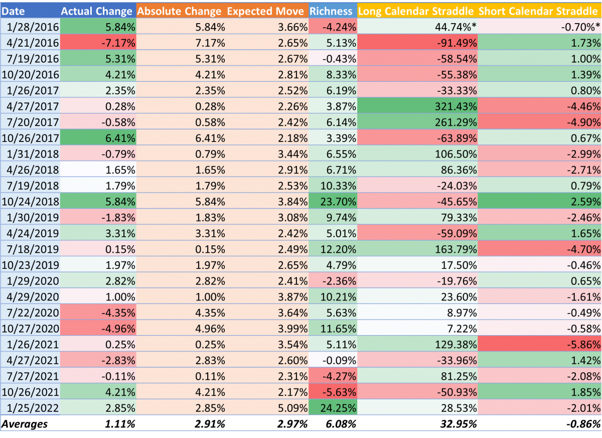
Consider the earnings moves for Microsoft ($MSFT) from 2016 through early 2022. Note that this series of earnings will be used extensively throughout this analysis because $MSFT is a large company with strong option liquidity. They also had a wide range of earnings results relative to post-earnings movements and different IV environments.

Actual Change represents the realized post-earnings move in the stock after one day. Notice how the size and direction of these moves are relatively unpredictable. Over the course of 25 earnings, the range of moves is from down over 7% to up over 6% with no obvious patterns. They did, however, average over a 1% gain overall.

Absolute Change is the absolute value of the change. This stock averaged a nearly 3% move one way or the other after the earnings releases in scope.

30d IV is the 30-day IV for MSFT immediately preceding the earnings announcement. Note that this is an annualized rate based on the option IVs expiring near 30 days out.

Periodic IV is the single day IV derived from the 30d IV. Think of this as the 30d IV “uncompounded” from its annualized rate to a single day.

Expected Move is the breakeven move implied by the option prices (double the periodic IV).

Error is the difference between the absolute change and the ATM expected move. The more green, the more the magnitude of the actual move exceeded the expected move.

Like the overall change numbers, the differences between the expected move and the actual move are unpredictable. However, the average turned out to be almost exactly on target with a mean error of just -0.05%. This negligible error indicates that—in aggregate—options have been priced nearly to perfection. So is there any opportunity here?

What about trading earnings directionally with options?

Over the term in focus, Microsoft rose an average of 1.11% the day after announcing earnings results. This would indicate that there might be some opportunity to trade directionally using options from the same term.

Here’s what the standard ATM option trades would have returned if each position were opened using the pre-announcement closing prices and closed using the post-announcement closing prices. The data below assumes market pricing such that all buys executed at the ask and all sells executed at the bid.

Unsurprisingly, bullish trades did better when the underlying price rose and fared worse when it dropped. However, it’s important to note that of the 17 times the stock rose after earnings, the ATM long call only appreciated in value 10 times. While some of this could be attributed to liquidity costs, the substantial difference of the average 1.11% return on the stock relative to the -5.66% return on long calls indicates that there’s much more at play. At the same time, selling puts instead of buying calls turned out to be a much more effective long strategy as it was profitable 21 times—including 4 times when the stock itself dropped—for an average return of 4.23%. Note that the short trades use the appropriate naked short margin requirement as the investment basis for each return.

How do we compare returns of long and short strategies?

While it may be tempting to compare inverse long and short trade returns, it’s not as easy as it seems. All of the trades in use here are naked trades in that they’re all uncovered. While the term “naked” is most often associated with uncovered short positions, it also applies to long positions that don’t have corresponding short positions, especially for our purposes.

Comparing the returns on naked trades is complicated because they’re missing key data for practical purposes. Naked long positions have an unlimited maximum return for all practical purposes. While this isn’t technically true for long put positions, it effectively applies here as there’s no feasible value to use for its maximum return as the underlying is not expected to actually go to zero immediately following the earnings release. Without a maximum potential profit value, you can’t calculate how effectively the trade capitalized on the total opportunity like you could with a defined return trade.

The situation for short trades is similar in that while they both have well-defined maximum potential profits, they don’t have a practical cost basis. Like the issue with long puts above, the underlying cannot be expected to go to zero during our timeframe, so using the strike as an investment basis won’t offer useful results. Instead, short calls and puts use their naked margin requirement as the investment basis. The short straddle uses the greater margin requirement of the call and put legs. As a result, the maximum possible rate of return is the net profit relative to the margin requirement. In the cases where the corresponding puts or calls went to zero after earnings, the trade fully capitalized on the opportunity, but never reaches even 15% due to the high margin requirement used as the investment basis.

Given all of the above, the practical guidance is to use the total averages to evaluate how each strategy performed in aggregate over the course of the analyzed term. It’s not a perfect solution since each short trade strategy doesn’t have the same maximum potential return each time, but it’s good enough to understand the relative performance of each overall strategy.

How important is option liquidity?

As mentioned earlier, liquidity is a key factor when considering options trades. In the options world, liquidity describes how easy it to enter and exit positions that express precise views. There are a lot of factors that come into play, including the number of option terms, the width of strikes available, typical volume, and open interest. However, the most important factor for the earnings trades we’ll cover here is the bid/ask spread. The wider it is, the more expensive it can be to enter and exit a given position because you’ll need to take a hit on the liquidity premium. For example, an option with the spread 0.95/1.05 may have a fair value of 1.00, but the spread could cost you 5% each time you trade it if you want immediate fills.

In order to minimize the impact of liquidity on our analysis, we’ll use midpoint pricing moving forward. This isn’t an ideal approach because it gives an unrealistic expectation as to the net returns, and it usually implies better returns that you’d probably get. However, our focus here is on the relative returns of trades to each other, so the absolute numbers aren’t as important.

Also, during market hours, near-term ATM options for $MSFT generally trade with penny spreads such that the 1.00 option from earlier would be priced 0.99/1.00 or so. However, our analysis uses end-of-day (EOD) market prices, so the spreads will be a bit wider. Using the midpoint is probably a better approximation of the kinds of returns that would have been seen during peak market hours.

Now let’s take a look at the returns for the trades above using midpoint pricing.

You might have noticed that the average returns for both long and short calls were positive. This is a peculiar side effect of the way naked short returns are calculated as described earlier. Obviously the net gains from the long call strategy exactly equal the net losses for the short call strategy. But since they use different methodologies for calculating the investment bases their returns are derived from, the returns don’t line up perfectly. While the short call strategy would have produced a net loss had it been equally weighted across terms, the nature of averaging trade returns that aren’t exactly equal produced this slightly misleading result.

While all of the returns are understandably better than those shown earlier, they still tell the same general story about how the short directional or straddle trade outperforms its long counterpart (selling puts vs. buying calls). Why exactly does selling options outperform? The answer is IV crush.

What is implied volatility crush (IV crush)?

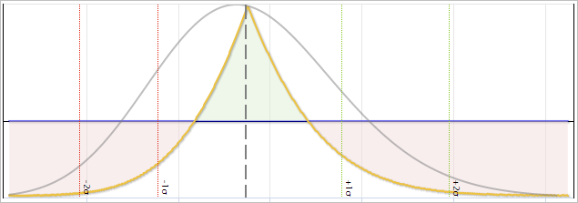
Implied volatility is the measure of how uncertain the outcome of a given option will be leading into its expiration. It can change over the course of its lifetime as certainty increases or decreases due to virtually any reason. When certainty increases drastically—such as when an earnings report is disclosed—the market has an opportunity to reset expectations for the underlying with greater confidence. This increased confidence means that there is less risk due to unknowns, so implied volatility drops almost immediately.

This drop is known as IV crush and is expressed as the percentage of IV retained by an option after the event occurs. For example, an option with an IV of 50% ahead of earnings may drop to 35% after the announcement. In this scenario, the crush rate is calculated as $latex \frac{35\%}{50\%}=70\%$.

What is earnings IV crush?

IV crush almost always happens immediately after each earnings announcement and is usually in the 50-90% range for the 30-day IV. Of course, this earnings IV crush is subject to the circumstances of the market and underlying. Investors new to options often bemoan the impact of IV crush, especially after earnings.

The story is always the same. An investor has a directional view, so they buy calls or puts to express it. They turn out to be right about the direction but are shocked to discover that the options aren’t worth nearly what they expected them to be worth when the market opens. This is because the uncertainty was cleared up in the earnings release, leaving a much more predictable range of outcomes for the underlying. This predictability means that IV gets crushed and many options may end up only being worth their intrinsic value. If the underlying didn’t quite move enough to make up for the crush, then the investor could end up being correct and still lose money. It’s become a rite of passage for many on forums like Reddit. It’s also the explanation as to why short option strategies outperformed long option strategies during the earnings periods discussed earlier.

This isn’t necessarily an argument against making directional earnings plays with options. Instead, it’s a reminder that with options you need to not just be right about direction, but also magnitude and timing. In the meantime, the clock is ticking away and the time value for long options (measured as theta) keeps slipping away.

How much does IV crush after earnings?

Here are the actual crush numbers for IV around recent Microsoft earnings.

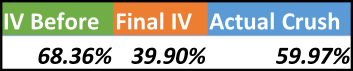
IV Before is the IV for the nearest option term on the last pre-earnings trading day. The nearest IV expiring after earnings is also referred to as the earnings IV. Note that this IV is derived purely from the options at this term, unlike the 30-day IV, which is usually blended from options straddling the 30-day horizon.

Final IV is the earnings IV on the first post-earnings trading day.

Actual Crush is the crush rate observed by dividing the post-earnings IV into the pre-earnings IV. Earnings IV crush is expected to be substantially more impactful than the crush applied to the 30-day IV, hence the lower rate of IV retained.

As IV is almost always elevated going into earnings, it can be expected to drop after the uncertainty is cleared up. However, in some cases the earnings results may introduce concerns about the underlying, so there are occasionally increases in IV as the market shifts from earnings uncertainty to uncertainty around something disclosed in the earnings release. As a result, the highest crush rates (the times when IV contracted the least) usually coincide with disappointing earnings where the stock drops afterwards.

Can we predict the earnings IV crush?

Historically, the market has used the long-term IV as a predictor for the level IV will settle into after an earnings report. While short-term IVs are heavily correlated with the next earnings release, long-term IVs look out over a period of quarters—or even years—during which there will be many events to consider. As a result, they don’t tend to elevate much as near-term announcements approach.

Here’s a comparison of how effective long-term IV has been at predicting the IV crush for near-term IV.

Long Term IV is the IV for the farthest available option term on the last pre-earnings trading day.

Implied Crush is the crush rate implied by dividing the farthest IV into the nearest IV before earnings.

Actual Crush is the observed crush after the earnings announcement.

Actual vs. Implied is the actual crush less the implied crush. In almost every case, the long-term IV underestimates the size of the crush. This is partly because the long-term IV includes many events over the course of years, whereas the remaining earnings IV is often just a few hours or days with little news expected.

Can we infer anything from the volatility surface?

Beside the long-term IV, options investors also look at the volatility surface to better understand the perceived risk around earnings. The volatility surface is simply the mapping of all option volatilities across all terms in a single view. Whereas the IVs for a given term can be easily mapped on a 2D surface to provide the volatility skew, extending and connecting multiple skews across different terms creates a 3D model known as the volatility surface. The peaks and valleys of the surface are often used to identify where the market is pricing options more or less than might be expected relative to nearby strikes or terms.

While the surface can’t tell you what IV will crush to after earnings, it can tell you what the market is pricing options to crush to. After all, if there are prevailing prices for the options at the same strike across different terms, there must be a price at which a calendar trade breaks even.

For example, consider two ATM calls trading at the same strike one week apart and both expiring after the next earnings call. If you sell the front week and buy the back week, it’s possible to determine various scenarios at which the trade will break even based on experimenting with different underlying prices and IV after the earnings announcement. Since both options have the same strike, underlying price changes (delta) will cancel out, so the week one call will lose value faster than the week two option—unless the changes in IV are inconsistent. Identifying exactly what those IVs are yields the earnings IV crush rate implied by the market.

Earnings Crush Rate is Quantcha’s proprietary measurement of the crush rate being priced by the market for the first ATM options expiring after earnings. The higher the rating, the more IV the ATM options are expected to retain after the announcement. However, like the other crush rates, these are measured relative to the options that are ATM at the time, which may be different options depending on how much the underlying price moves.

Actual vs Crush Rate is the actual crush rate less the Earnings Crush Rate. The lower this rate, the more the ATM IV crushed beyond the market pricing.

It’s important to understand that the Earnings Crush Rate isn’t a guarantee of what the rate will crush to. Instead, it’s the inference of what the market is pricing it to crush to after earnings based on the volatility surface. The higher this rate is, the less the market is pricing earnings IV to crush by. However, to better gauge the magnitude of the premium it’s useful to compare the rate—or at least the IV the rate implies—to estimate the size of the opportunity. Since we can usually expect the earnings IV to crush below the long-term IV, it’s a good candidate for comparison. By subtracting the long-term IV from the crush-implied IV, we can produce a richness rating.

Crush Implied IV is the pre-earnings IV multiplied by the Earnings Crush Rate. This is what the post-announcements earnings IV is priced to drop to.

Richness is the crush-implied IV less the long-term IV. The higher the richness, the more premium the earnings options are demanding relative to the expected IV indicated over the long term. If the earnings IV ultimately crushes to (or below) the long-term IV, which is usually does, then the pre-earnings IV will have been overpriced relative to the rest of the surface.

Can we still lose by selling overpriced IV?

In short, yes. The nature of IV is that it represents the risk of a move of a certain magnitude in the underlying asset. When we determine that IV is overpriced, what we’re really saying is that the probability of a large enough move to justify the breakeven price is not worth the cost of the options. In many cases this isn’t really feasible by using option prices alone. After all, the risk is measured from IV derived from option prices, which are calculated based on the perceived risk. It’s a self-regulating loop. If the market thinks that IV is overvalued, then it gets sold. This action drives down option prices, in turn driving down IV until it reaches equilibrium with the market consensus.

However, none of this means that the probability of an outsized move is out of the question. It’s always possible for an overpriced option to appreciate in value, so the notion of blindly selling options to capitalize on IV crush isn’t always going to work. However, the data from earlier indicates that selling naked earnings straddles for MSFT would have produced a net profit averaging 5% over the past 25 earnings releases, so the numbers appear to be in favor. The only time the trades lost big were when the underlying move substantially beyond the move implied by IV.

How can we hedge against directional moves?

The basic strategies covered so far have been effective in illustrating the nature of earnings trades using some simple option approaches. However, despite the fact that the underlying moved up following most of the earnings, it’s clear that the real winner has usually been selling IV against the impending crush. However, there were enough outsized moves to blow naked shorts out of the water often enough to substantially dampen long-term average returns.

So the new question becomes, how can we sell IV while simultaneously hedging against those outsized directional moves? Thanks to the versatility of options, there are a lot of ways.

Iron butterflies

The most obvious answer is to hedge the short call and put by buying corresponding calls and puts. This caps your risk and provides a defined potential return.

The downside of this trade relative to short straddle is that the cost of the hedging options eats away at potential profit. Plus, since both options are OTM, they’re both entirely paying for time value and one will almost surely end up worthless.

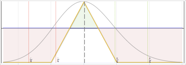
Short strangles

A similar strategy to the short straddle is the short strangle. It provides a way to sell IV while partially hedging against an outsized move by sliding strikes farther out of the money (OTM). For example, instead of selling ATM options where one side will definitely be in the money the next day, you can sell a strangle that combines a short OTM call and a short OTM put.

The farther the strikes are from the money, the more likely both will still be OTM after the earnings move. The downside to this strategy is that the time value premium collected decreases rapidly as strikes get farther from the money, so one big loss could wipe out profits from several complete wins.

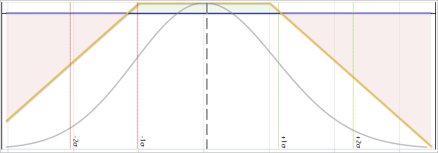
Iron condors

If you combine the logic behind the short strangle and iron butterfly strategies, you end up with the iron condor. It provides good hedging by widening the area for maximum profit while also capping risk.

However, these hedging compromises mean that not only are you accepting less credit to open, but you’re also paying for insurance. In these cases, it’s critical that the underlying not breach the short strikes as the costs of managing iron condors around earnings can be very expensive unless everything comfortably expires on its own.

The problem with single-term trades

The strategies discussed in this section can help you capitalize on profit from overpriced IV while hedging against an outsized move in the underlying. However, they all include their own directional risks. As a result, they’re not really “short IV” strategies as much as they’re “undersized move” strategies. Despite having near-zero deltas and gammas, these strategies don’t do a great job of isolating the IV opportunity because their profits are entirely centered on the expectation that the underlying will move less than the IV implies it will.

The concepts discussed during the IV crush section focused on how the crush for earnings IV occurs within the context of the rest of the volatility surface. In other words, capitalizing on the overpriced IV in the shortest-dated options can only really be directionally hedged with options expiring on a later date or else they would be surrendering the IV advantage as all options for a given date are subject to the same elevated IV. Strategies making use of options expiring across different terms are known as calendar trades.

How do calendar trades hedge out directional risk?

Option prices can be broken down into two different components: intrinsic and extrinsic.

Intrinsic value is based on how deep the options are in the money (ITM). In other words, this represents the value of immediate exercise. If a stock is trading at $110, all of its call options struck at 100 have $10 of intrinsic value per share, regardless of when they expire. All OTM options have an intrinsic value of 0.

Extrinsic value is also known as time value and represents everything that gives the option value besides its intrinsic value. This value is based on a combination of the factors that drive uncertainty around whether or not the option will expire ITM. In other words, options that are virtually guaranteed to expire in or out of the money will have no extrinsic value. The highest extrinsic value is always for options ATM.

Simply put: $latex fair\ option\ value=intrinsic\ value+extrinsic\ value$

As a side note, there is a third value that comes into play when evaluating the fair option value relative to its price: liquidity cost. The liquidity cost is the difference you pay or receive from the fair option value and is usually inferred from the bid/ask spread. Since we’re working with midpoints here, the option price is considered the same as the fair option value.

Consider a trade where you are short one near-term call at 100 and long another longer-term call at 100. Assume there are no underlying dividends to account for. As the underlying moves up or down, the intrinsic value of both options remains the same because they are struck at the same price.

Although they have the same intrinsic value, the options likely have slightly different deltas as the shorter-dated option is more sensitive to underlying price movement. But that’s not because its intrinsic value changes more. It’s because the likelihood of the option being ITM at expiration changes more from underlying price movement. Longer-dated options provide more time for the underlying to move, so their deltas will be lower.

Given that they have the same strike, the shorter-dated call will also have a higher theta. This means that its time value will erode faster than the time value of the longer-dated call as the ITM uncertainty drains faster.

If the IV of the near-term call drops more than that of the long-term call (as we expect from earnings IV crush), then we’ll also see an outsized decrease in value there, as well. Since we’re short the near-term call, this will play to our advantage.

How can we employ calendar trades to capitalize on IV crush?

The most effective strategy for capitalizing on earnings IV crush trades is the calendar straddle. Put simply, this strategy involves selling the ATM straddle for the overpriced term while buying that same straddle for the underpriced term. When the long straddle is taken for the later week, the strategy opens with a net debit and is the long calendar straddle. Buying the near week and selling the far week produces a net credit and is the short calendar straddle. In either scenario, the directional moves cancel out since the strikes are identical, so the profit opportunity comes from changes in the time value/IV component of the option prices.

Since we have some metrics to determine when the earnings week IV is relatively overpriced (which is pretty much always), pairing those positions with their inverse counterparts on a future week (like the following expiration) provides near-complete directional hedging.

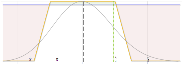
Employing a long calendar straddle provides a P&L optimized for outsized profits when the underlying moves less than the IV implies. However, while it loses money when the underlying moves more than anticipated, those moves are largely dampened by the net gain in IV crush. It’s also important to note that while this trade shares a similar shape to that of the short strangle or iron butterfly, its investment basis tends to be much lower as the cost of the far straddle is usually not substantially more than the credit received for the near straddle.

Long calendar straddle profitability

The fair value of a calendar straddle is simply the difference in extrinsic value between the long and short straddles. This means that profit happens when that difference grows between the times you buy and sell it. Since we know that the extrinsic value of the short straddle will approach zero after earnings, we’re relying on the long straddle retaining enough time value to exceed the net debit paid to open the overall strategy.

If the underlying doesn’t move much, then all options are still near the money, which means they’ll retain the most extrinsic value. However, since both the IV crush and percentage of time remaining impact the short week much more, the result should be a substantial profit.

On the other hand, if the underlying makes an outsized move, it usually results in an overall loss. A sharp move down, for example, would drive the price of both calls to zero and the puts to their intrinsic value. The extrinsic value of all options here zeros out because they’re either deep in the money or deep out of the money.

Profit from moves close to the expected magnitude will depend on a variety of factors. For example, a downward move within range should wipe out all value from the short call but may leave a small amount to be salvaged from the long call. While both put legs will increase in value, the short put will approach intrinsic value while the long put will hopefully retain some time value. The more the expiration week was overpriced, the more likely the trade will be profitable.

In our analysis, long calendar straddles produced a remarkably outsized average gain for the $MSFT earnings releases in scope here.

*Note that the EOD midpoint pricing for the Jan 2016 trades indicated the long calendar straddle could be opened for $0.01 due to an infeasibly high put ask at the near expiration. To account for this, trades using that option were priced at the near put bid. This adjustment drastically lowered the long return and slightly raised the short return.

The long calendar straddle strategy was profitable 14 of the 25 earnings periods analyzed here for an impressive average return of nearly 33%. In fairness, this is using midpoint pricing, which is probably too optimistic. However, it gives a more realistic view of option pricing than the EOD bid/ask spread leading into earnings. It’s also important to recognize that the average long calendar straddle had an opening cost of just 0.78% of the underlying stock price. In other words, if the stock were trading at $100, the typical long calendar straddle at close before the earnings announcement was just $0.78/share.

Trade profitability was clearly dependent on the magnitude of the underlying move relative to its expected move. On average, they were virtually the same at 2.91% vs. the expected 2.97. As a result, the strategy was profitable 11 of the 13 times the actual move was less than the expected move. There are a variety of reasons why those trades could have lost money in their respective scenarios that include issues like lower IV crush than expected, poor option liquidity, or earnings IV richness.

Another important detail here is that the trade was profitable 3 of the 12 times the actual move exceeded the expected move. This was likely due to higher IV crush, better option liquidity, or more favorable earnings IV richness. This also explains how the trades still retained a fair amount of value even when the actual move drastically exceeded the expected move.

A note about calendar strangles

A close cousin to the calendar straddle is the calendar strangle. It’s the same conceptually, except that the call and put strikes are both OTM instead of ATM. While calendar strangles also profit from IV crush, our analysis found them to be less successful overall due to substantially higher time value lost in the long strangle component. However, if there is strong evidence that the underlying will make an outsized move in either direction, picking the correct strikes for a calendar strangle should outperform the calendar straddle.

How does this analysis hold up across the broader market?

The data used so far in this analysis was limited to the 25 earnings releases for $MSFT from 2016 through early 2022. To consider how these results hold up across the broader market, we expanded the analysis to include all optionable US equities. The only refinement applied was to cull out stock that didn’t have strong option liquidity in order to focus on realistic market opportunities and minimize the impact of midpoint pricing.

To perform this filter, we only used earnings releases for stock that had a Quantcha Liquidity Rating of 4 or higher on the last trading day before the release. This rating evaluates the option liquidity for stocks on a daily basis and includes factors such as the number of option terms available, distance between option strikes, volumes, open interests, and the bid/ask spreads.

The final result produced 1,097 earnings releases across 434 stocks between 2016 and the beginning of 2022. The qualifying releases skewed toward the more heavily traded stocks and toward more recent releases, although quite a few smaller stocks also made the cut if their options were heavily traded. About 15% of the releases were for stocks that only had one qualifying release make the cut.

Among these releases, the average 1-day return for the underlying was around 50bps, although the average magnitude of the change was nearly 5%. Option volatility was slightly underpriced across these releases with an error of 37bps, which likely indicates that there was often significant interest in selling IV from the market.

Given the market’s support for selling IV, earnings IV was much less exaggerated going into announcements. As a result of these tempered numbers, earnings IV only crushed to 60% on average. However, that doesn’t mean that there wasn’t real opportunity.

The first six trades above reference trading the ATM earnings options. The calendar trades combine the earnings straddles with the inverse position at the next expiration.

Unlike the $MSFT trades, it appears that the better way to have traded bullish returns was via long calls (as opposed to short puts). This likely indicates that IV was underpriced going into earnings when the underlying ultimately enjoyed a bullish move.

On the other hand, the more effective bearish trade was to sell calls, which suggests that IV tended to be exaggerated in cases where the underlying ultimately dropped after earnings. Obviously, these sorts of conclusions are easy to presume in hindsight, so this is more speculation than actionable insight.

The most striking data point, however, is the outsized rate of return for the long calendar straddle. While not quite the 33% seen for $MSFT earnings, it still averaged nearly 13%. This suggests that the opportunity to profit off of earnings IV crush may be consistently available even when earnings IV. The trade was profitable around 53% of the time with an average return of 66% when profitable.

Key conclusions

This report highlights some of the opportunities that exist when using options to trade earnings results. Here are some of the key conclusions we’ve come to in the process of researching it.

Earnings IV crush is real and has been the most substantial and reliable opportunity lately. Strategies focused on selling IV outperformed other types of trades most of the time, regardless of the ultimate move of the underlying. Data like IV across different terms and Quantcha’s Earnings Crush Rate can help derive a richness metric to identify special opportunities on a case-by-case basis.

Naked directional trades are generally not worth the risk. Most of the earnings releases in scope occurred during a bull run, but bullish option trades didn’t generally pay well during the period. This doesn’t invalidate the notion of using directional option strategies when expressing a directional view, but simply buying calls during a bull run earnings period shouldn’t be assumed to outpace an underlying position. Even when you’re right about direction, you’ll still need to be right about timing and magnitude to see a profit.

Option liquidity is an extremely important factor. Although option liquidity tends to be highest for stocks leading into their earnings releases, it’s not necessarily a guarantee of great pricing. As the strike moves further from the money, there will be fewer market participants willing to take the other side of your trade, so consider data like the Quantcha Liquidity Rating to locate opportunities worth pursuing.

Data used in this research

Much of the volatility data used for this research came from Quantcha’s US Equity Historical & Option Implied Volatilities database available through NASDAQ. It’s updated daily and includes over 60 daily volatility indicators for historical and implied volatilities across terms ranging from 10-day to 1080-day (3-year), as well as skew steepness measurements.

The Earnings Crush Rate and Liquidity Ratings used here came from Quantcha’s US Equity Option Ratings database available through NASDAQ. It’s also updated daily and includes key option-derived data points for earnings, option liquidity, and IV valuation ratings like IV Rank, IV Percentile, and Quantcha’s proprietary IV Rating.

About Quantcha

Quantcha provides tools, data, APIs, and research for some of the world’s leading financial institutions, including top hedge funds, market makers, and quantitative traders. The Quantcha Options Suite has been featured in prominent trade publications for its innovative approach to the full options portfolio management lifecycle, including integration with major brokerages like Charles Schwab’s TD Ameritrade, Morgan Stanley’s E*TRADE, Tradier, and more.

For more information about custom tools, data, APIs, or research, please reach out to us at hello@quantcha.com.